Advertisement
Help Keep Boards Alive. Support us by going ad free today. See here: https://subscriptions.boards.ie/.
https://www.boards.ie/group/1878-subscribers-forum
Private Group for paid up members of Boards.ie. Join the club.
Private Group for paid up members of Boards.ie. Join the club.
Hi all, please see this major site announcement: https://www.boards.ie/discussion/2058427594/boards-ie-2026
The Sudden Stratospheric Warming
-
02-11-2009 09:06PM#1


Comments
-
-
-
-
-
-
Advertisement
-
-
-
-
-
-
Advertisement
-
-
-
-
-
-
-
-
-
-
-
Advertisement
-
-
-
-
-
-
-
-
-
-
Advertisement
-

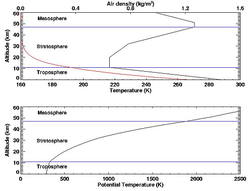 shows a typical vertical profile of density from the ground to 60 km. The density of air near the top of the stratosphere is nearly zero.
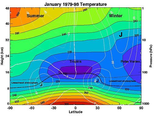 shows a color image of zonally-averaged January temperatures from the South Pole to the North Pole and between the surface and 48 km (158,000 feet), averaged from 1979-1998. The tropopause is superimposed on Figure 6.02 as the thick black line. The tropopause is highest in the tropics, and lowest at polar latitudes.
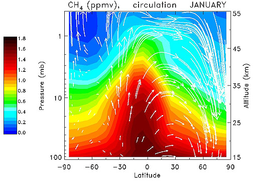
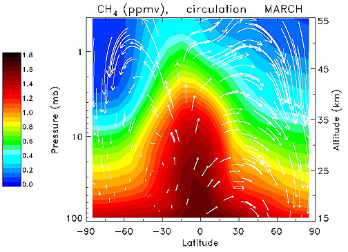
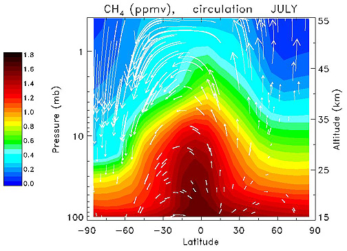
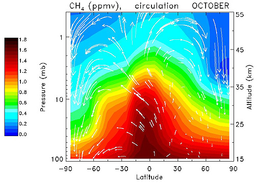 show methane distribution for January, March, July, and October respectively. Methane has its source region in the troposphere, and is lost in the stratosphere by a reaction with OH molecules and oxygen atoms.
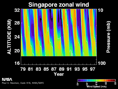
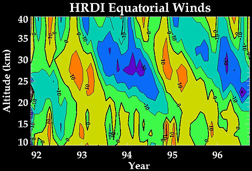
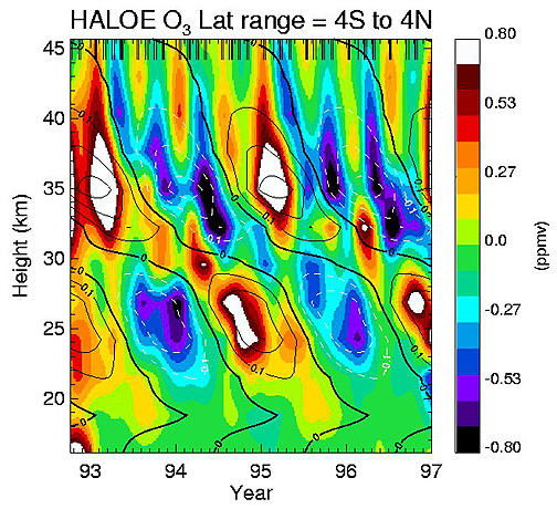 shows these ozone anomalies versus altitude for the 4°S to 4°N region. The data is based on the UARS HALOE instrument, with reds denoting high ozone and the blues denoting low ozone. In this figure, the time average has been subtracted out. Superimposed on the ozone anomalies in the black contours are the HRDI zonal winds.
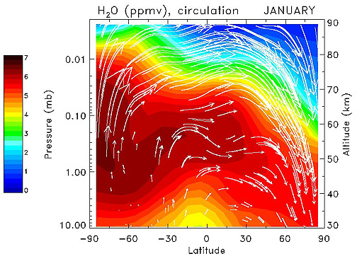 shows this circulation in the stratosphere and mesosphere, superimposed on the water vapor distribution for January (northern winter/southern summer).
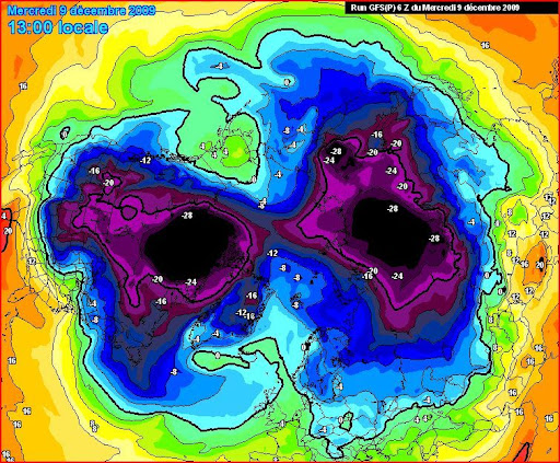
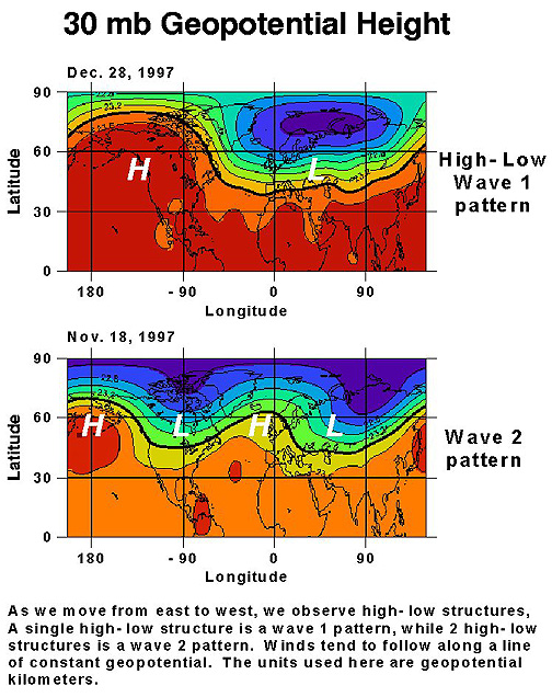 which shows a weather map for the stratosphere at the 30 mb geopotential height level (about 23 km altitude). The wind tends to blow along the lines of constant geopotential height. (Geopotential height is defined and discussed in Chapter 2.) The top image shows the height field on December 28, 1997. The bottom image of Figure 6.14 shows the same 30 mb geopotential height field on Nov. 18, 1997.
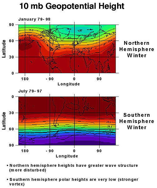 which shows the climatological average winter geopotential height distribution for the northern hemisphere (January) and the southern hemisphere (July) at 10 mb or about 32 km altitude. The northern winter is based on 1979-1998 January data, and the southern winter is based on 1979-1997 July data.
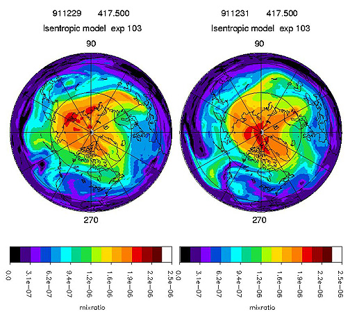 shows northern hemisphere ozone mixing ratios from a 3-dimensional transport model on the 417 K (144°C or 291°F) isentropic surface for December 29, 1991 (left) and December 31, 1991 (right). The high ozone levels over the polar region are within the polar vortex which persists throughout the winter.
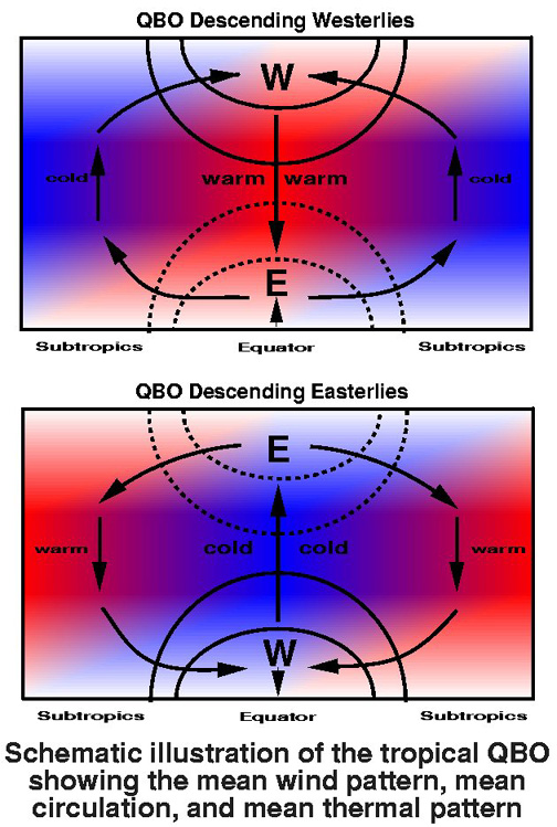
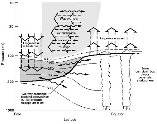 shows schematically these two layers of the stratosphere and the dynamical processes that occur in each.

![[Deleted User]](/applications/dashboard/design/images/defaulticon.png)


Advertisement